The Role of Optimization Algorithms:

Neural networks are composed of layers of interconnected neurons, each with adjustable parameters. These parameters are initially set randomly and need to be fine-tuned during training. This fine-tuning is achieved by optimizing a loss function, which quantifies the error between the model's predictions and the actual target values.

Optimization algorithms are responsible for iteratively adjusting these parameters to minimize the loss function. The journey to the optimal set of parameters can be challenging, as the loss landscape of deep neural networks is often complex, with numerous local minima and plateaus. The choice of optimization algorithm greatly influences the speed of convergence and the final performance of the model.

We’ll look into different types of optimizers and how they exactly work along with their specifications.

1. Gradient Descent

2. Stochastic Gradient Descent (SGD)

3. Mini Batch Stochastic Gradient Descent (MB-SGD)

4. SGD with momentum

5. Nesterov Accelerated Gradient (NAG)

6. Adaptive Gradient (AdaGrad)

7. AdaDelta

8. RMSprop

9. Adam

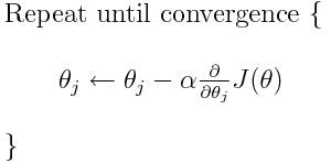
1) Gradient Descent

Gradient Descent calculates the gradient of the cost function concerning these parameters. The gradient indicates both the direction and magnitude of the steepest ascent of the cost function at the current parameter values.

The algorithm then updates the parameters in the opposite direction of the gradient, using a hyperparameter known as the learning rate to control the step size. This step-size adjustment ensures that the optimization converges effectively without overshooting or taking excessively small steps.

Changing learning rates impact on gradient descent

This iterative process continues until a predefined stopping criterion is met. Common stopping criteria include reaching a maximum number of iterations or achieving a certain level of loss, indicating convergence.

However, it's essential to be aware that Gradient Descent can sometimes get trapped in local minima, points where the cost function is lower than in the immediate vicinity but not necessarily the global minimum. To address this issue, variants of Gradient Descent, like stochastic gradient descent (SGD) introduce randomness and adaptive learning rates to escape local minima and accelerate convergence.

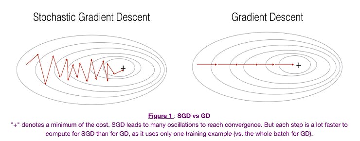
2) Stochastic Gradient Descent (SGD)

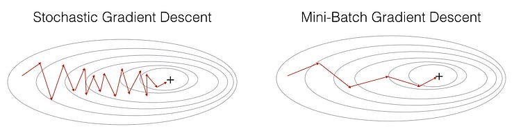
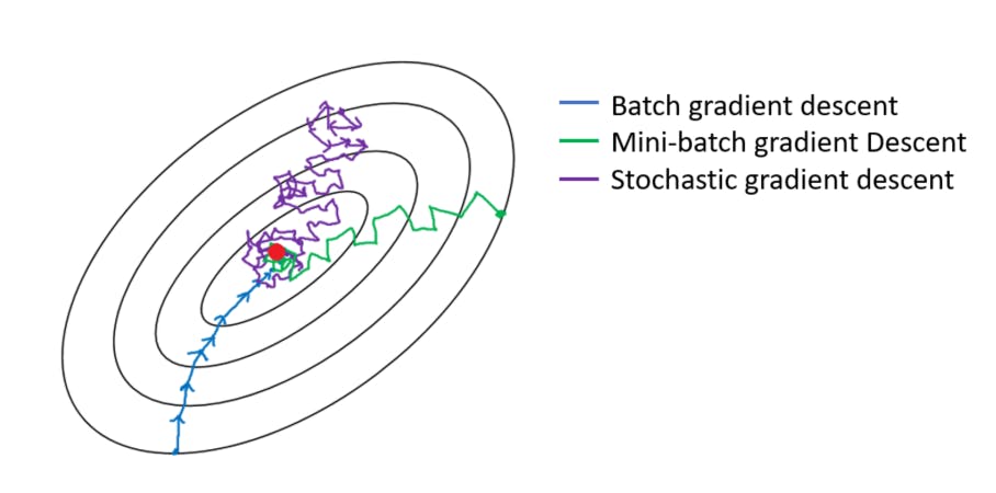
SGD differs from standard Gradient Descent in the way it updates model parameters. Instead of computing the gradient of the loss function using the entire dataset, as in Batch Gradient Descent, SGD computes the gradient using only a single randomly selected training example (or a small batch of examples) at each iteration. This introduces randomness into the optimization process.

Key characteristics and advantages of SGD:

1. Efficiency: SGD is computationally more efficient because it processes one or a few data points at a time, making it suitable for large datasets. This mini-batch processing helps speed up convergence.

2. Stochasticity: The randomness inherent in SGD can help escape local minima in the loss landscape, making it more resilient to getting stuck in suboptimal solutions.

3. Faster Convergence: SGD's frequent parameter updates can lead to faster convergence, as it quickly adapts to changing gradients.

However, SGD also has its challenges:

1. Noisy Updates: Due to the randomness of individual data points, SGD's parameter updates are noisy, which can result in oscillations during training.

   

2. Learning Rate Tuning: The learning rate is a crucial hyperparameter in SGD. It must be carefully tuned, as too large a learning rate can lead to divergence, while too small a learning rate can cause slow convergence.

3. Lack of Smoothness: The random selection of data points means that the loss function may not decrease smoothly over time.

To address some of these challenges, variants of SGD, such as Mini-Batch Gradient Descent, incorporate the benefits of both SGD and Batch Gradient Descent by using small, randomly sampled batches of data for gradient computation.

3) Mini Batch Stochastic Gradient Descent (MB-SGD)

MB-SGD algorithm is an extension of the SGD algorithm and it overcomes the problem of large time complexity in the case of the SGD algorithm. MB-SGD algorithm takes a batch of points or subset of points from the dataset to compute derivate.

Advantages of Mini Batch Stochastic Gradient Descent (MB-SGD):

1. Efficiency: Unlike Batch Gradient Descent, which computes gradients using the entire training dataset, MB-SGD processes a mini-batch of data samples at a time. This results in a significant computational speedup, making it suitable for large datasets.

2. Reduced Noise: Pure SGD can exhibit noisy parameter updates because it processes individual data points one at a time. In contrast, MB-SGD leverages mini-batches, providing a more stable estimate of the gradient. This helps reduce the noise in updates and smoothen the convergence path.

   

3. Parallelization: MB-SGD is highly amenable to parallel processing. The mini-batches can be distributed across multiple computing units (e.g., CPU or GPU cores), enabling efficient utilization of hardware resources and further speeding up training.

How MB-SGD Works:

1. Initialization: MB-SGD begins with an initial guess for the model's parameters, usually set randomly.

2. Mini-Batch Selection: At each iteration, MB-SGD randomly selects a mini-batch of data from the training set. The mini-batch size is a hyperparameter that needs to be chosen based on factors like available memory and computational resources.

3. Gradient Computation: It computes the gradient of the loss function with respect to the parameters using the data samples in the selected mini-batch. This gradient represents the direction and magnitude of the steepest ascent of the loss function at the current parameter values within the mini-batch.

4. Parameter Update: MB-SGD updates the model parameters by moving them in the direction of the negative gradient. The update rule for a single parameter θ is similar to that in standard SGD:

   The learning rate controls the step size for the update.

5. Convergence: The iterative process continues until a stopping criterion is met, such as reaching a predefined number of iterations or achieving convergence to a desired loss level.

4) SGD with momentum

A major disadvantage of the MB-SGD algorithm is that updates of weight are very noisy. SGD with momentum overcomes this disadvantage by denoising the gradients. Updates of weight are dependent on noisy derivatives and if we somehow denoise the derivatives then covergence time will decrease.

The idea is to denoise derivatives using exponential weighting average that is to give more weightage to recent updates compared to the previous update.

It accelerates the convergence towards the relevant direction and reduces the fluctuation to the irrelevant direction.

Advantages of SGD with Momentum:

1. Faster Convergence: By incorporating the momentum term, SGD with Momentum accelerates convergence. It helps the optimizer to overcome small oscillations and navigate steep and narrow parts of the loss landscape more efficiently.

2. Reduced Oscillations: The momentum term smooths out oscillations in the gradient descent trajectory, leading to a more stable and predictable convergence path.

3. Escape from Local Minima: The accumulated momentum from previous iterations can help the optimizer escape local minima by providing the necessary "push" to move out of these regions.

Hyperparameter Tuning: To use SGD with Momentum effectively, you need to tune two key hyperparameters: the learning rate and the momentum term. The learning rate determines the step size for updates, while the momentum term controls the impact of accumulated momentum from past iterations. Finding the right combination of these hyperparameters is crucial for optimal training.

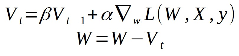
V(t) = γ.V(t−1) + α.∂(J(θ))/∂θ
θ = θ − V(t)

The momentum term γ is usually set to 0.9 or a similar value.

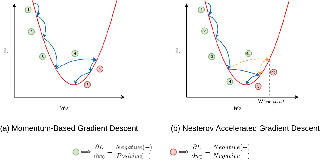
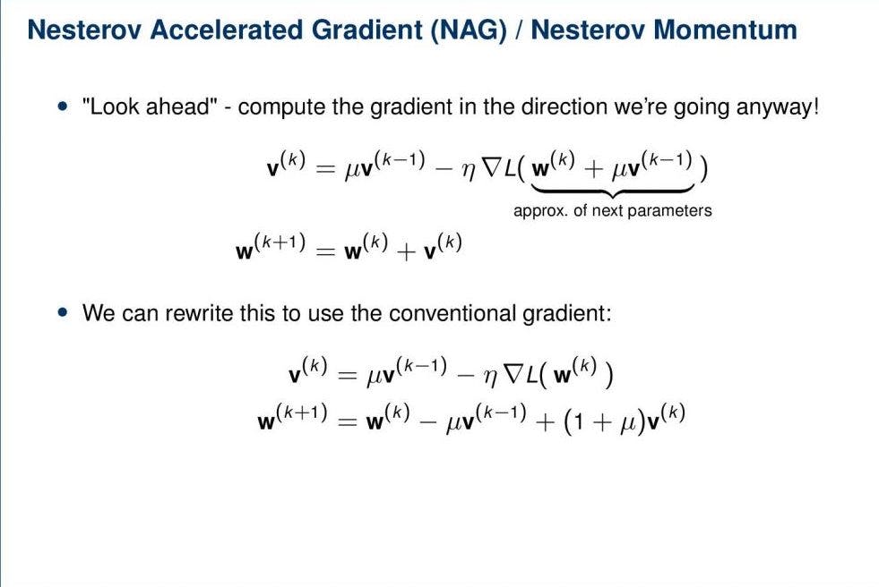
5) Nesterov Accelerated Gradient (NAG)

It is a variant of Stochastic Gradient Descent (SGD) with Momentum that further improves the convergence properties by fine-tuning how the momentum term is applied. Momentum may be a good method but if the momentum is too high the algorithm may miss the local minima and may continue to rise up. So, to resolve this issue the NAG algorithm was developed.

Key Features of Nesterov Accelerated Gradient (NAG):

1. Momentum: Similar to SGD with Momentum, NAG employs a momentum term (γ) to accelerate convergence and dampen oscillations. This momentum term represents a moving average of past gradients and is a hyperparameter typically set between 0 and 1.

2. Gradient Prediction: What sets NAG apart is its "lookahead" mechanism. Instead of applying the momentum term to the current gradient as in SGD with Momentum, NAG estimates the gradient at a future point (the point where it would be after applying the momentum term). It computes a gradient prediction by taking a small step in the direction of the current momentum

   

   Advantages of Nesterov Accelerated Gradient (NAG):

   1. Faster Convergence: NAG's lookahead mechanism enables it to more accurately estimate the gradient's direction, resulting in faster convergence compared to standard SGD with Momentum.

   2. Reduced Overshoot: NAG is less prone to overshooting the minimum because it anticipates the effect of momentum. This feature makes it more robust and efficient in navigating steep and narrow parts of the loss landscape.

   3. Improved Accuracy: The improved accuracy of the gradient prediction helps NAG achieve better final parameter values, leading to improved model performance.

Hyperparameter Tuning: Like other optimization algorithms, NAG requires careful tuning of hyperparameters, including the learning rate and momentum term, to achieve optimal results in training.

We know we’ll be using γ.V(t−1) for modifying the weights so, θ−γV(t−1) approximately tells us the future location. Now, we’ll calculate the cost based on this future parameter rather than the current one

V(t) = γ.V(t−1) + α. ∂(J(θ − γV(t−1)))/∂θ
θ = θ − V(t)

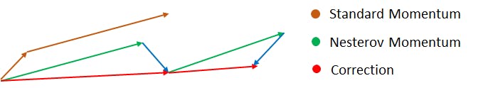
Again, we set the momentum term γ to a value of around 0.9. While Momentum first computes the current gradient (small brown vector in Image ) and then takes a big jump in the direction of the updated accumulated gradient (big brown vector), NAG first makes a big jump in the direction of the previously accumulated gradient (green vector), measures the gradient and then makes a correction (red vector), which results in the complete NAG update (red vector). This anticipatory update prevents us from going too fast and results in increased responsiveness, which has significantly increased the performance of RNNs on a number of tasks.

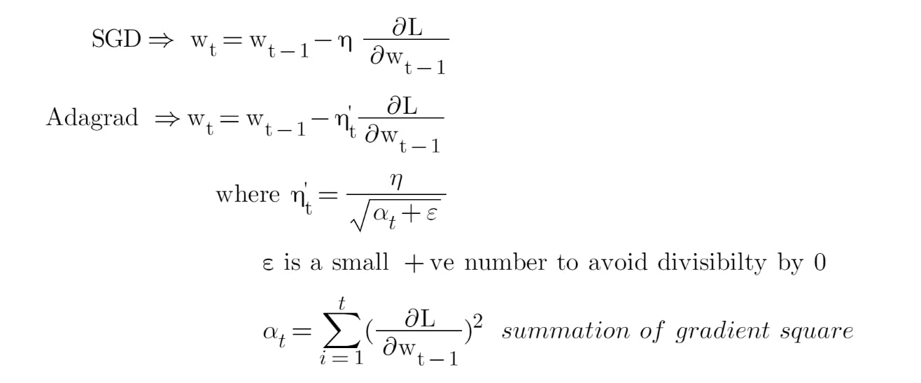
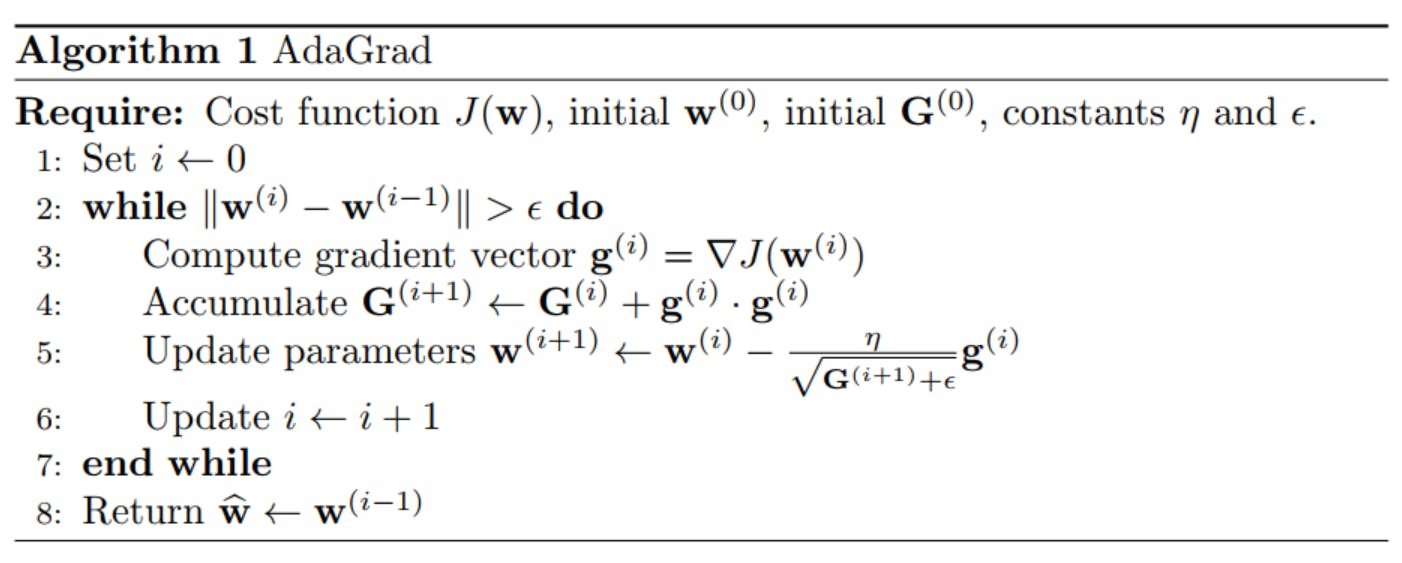
6) Adaptive Gradient Descent(AdaGrad)

It is designed to adapt the learning rate individually for each model parameter, improving the optimization process by automatically adjusting the step size based on the historical gradient information

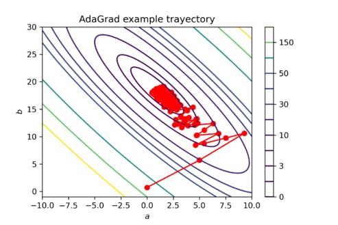
It performs smaller updates for parameters associated with frequently occurring features, and larger updates for parameters associated with infrequently occurring features.

Key Features of AdaGrad:

1. Individual Learning Rates: One of the main innovations in AdaGrad is that it assigns a unique learning rate to each model parameter. This adaptability enables the algorithm to handle situations where some parameters may require larger or smaller updates than others, which is especially useful when dealing with sparse data or highly varying gradients.

   

2. Gradient Accumulation: AdaGrad maintains a history of the squared gradients for each parameter. It does this by summing the squares of the gradients encountered during training. This accumulation of gradient information helps AdaGrad recognize which parameters have received larger or smaller updates, based on their historical gradient magnitudes.

Advantages of SGD with Momentum:

1. Faster Convergence: By incorporating the momentum term, SGD with Momentum accelerates convergence. It helps the optimizer to overcome small oscillations and navigate steep and narrow parts of the loss landscape more efficiently.

2. Reduced Oscillations: The momentum term smooths out oscillations in the gradient descent trajectory, leading to a more stable and predictable convergence path.

3. Escape from Local Minima: The accumulated momentum from previous iterations can help the optimizer escape local minima by providing the necessary "push" to move out of these regions.

7) AdaDelta

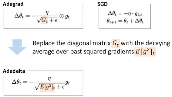
AdaDelta is an optimization algorithm designed to address some limitations of AdaGrad, particularly in scenarios with non-convex loss functions. Like AdaGrad, AdaDelta dynamically adapts the learning rates for each model parameter based on past gradient information, but it incorporates additional features to further enhance its performance and stability.

Key Features of AdaDelta:

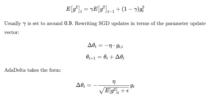
1. RMS Propagation: AdaDelta maintains two important moving averages for each parameter. Instead of accumulating squared gradients as in AdaGrad, AdaDelta computes the exponentially decaying average of squared past gradients, referred to as the "running root mean square" (RMS) of the gradient.

2. Adaptive Learning Rates: AdaDelta calculates an adaptive learning rate for each parameter using the RMS value. This learning rate adapts over time based on the past gradient information, but unlike AdaGrad, it does not accumulate the squared gradients indefinitely. Instead, it considers a limited history of gradients, making it more suitable for non-stationary and non-convex optimization problems.

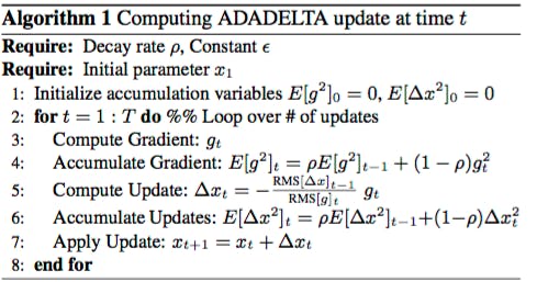
3. Parameter Update: The parameter update rule for AdaDelta is given by:

    Δθ = - (RMS(Δθ_t-1) / RMS(g_t)) * g_t
    θ_new = θ_old + Δθ
   

   Here, "g_t" represents the current gradient, "RMS(g_t)" is the RMS of the gradient, "Δθ_t-1" is the accumulated update history, and "θ" denotes the model parameter.

Advantages of AdaDelta:

1. No Learning Rate Hyperparameter: AdaDelta eliminates the need for a global learning rate hyperparameter, making it more robust and less sensitive to the choice of this hyperparameter compared to traditional gradient descent methods.

2. Adaptation to Non-Convex Loss Landscapes: AdaDelta's limited history of squared gradients helps it perform well in scenarios with non-convex loss functions where rapidly changing gradients can lead to divergent behaviour in AdaGrad.

3. No Manual Tuning: AdaDelta reduces the need for manual tuning of learning rates and hyperparameters, making it a user-friendly optimization algorithm.

Challenges and Considerations:

1. Memory Usage: Although AdaDelta uses a limited history of gradient information, it still requires some memory to store the RMS values for each parameter.

2. Complexity: The AdaDelta algorithm is slightly more complex to implement than standard gradient descent or AdaGrad.

In summary, AdaDelta is an adaptive optimization algorithm that overcomes some limitations of AdaGrad, making it well-suited for non-convex optimization problems. Its adaptability to learning rate changes and reduced sensitivity to hyperparameters make it a valuable choice for training machine learning models, particularly when dealing with complex, dynamic, and non-convex loss landscapes.

8) RMSprop

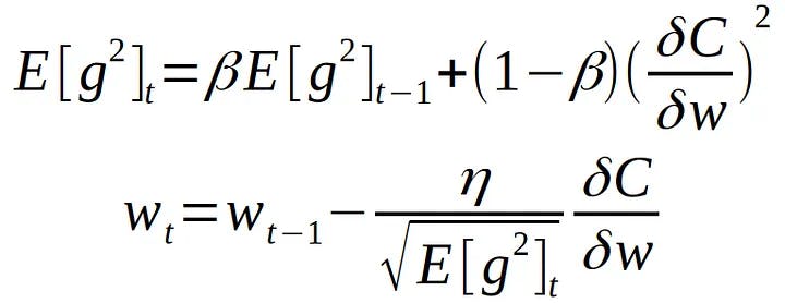
RMSprop adapts the learning rate for each parameter by computing the exponentially weighted moving average (EWMA) of the squared gradients. It divides the learning rate by the square root of this moving average, effectively scaling the step size based on the past gradient information. The formula for parameter update in RMSprop is as follows:

Δθ = - (RMS(Δθ_t-1) / RMS(g_t)) * g_t
θ_new = θ_old + Δθ

Here, "Δθ_t-1" represents the accumulated update history, "RMS(g_t)" is the root mean square of gradients, and "g_t" is the current gradient.

Advantages of RMSprop:

1. Adaptive Learning Rates: RMSprop automatically adjusts the learning rates for each parameter based on their historical gradient magnitudes. This adaptability is crucial for handling scenarios with varying gradients and complex loss landscapes.

2. Stability: RMSprop's division by the square root of the moving average of squared gradients helps stabilize the optimization process, preventing the learning rate from becoming too large and leading to divergence.

3. No Manual Tuning: RMSprop reduces the need for manual tuning of learning rates, making it a user-friendly optimization algorithm.

Considerations:

1. Memory Usage: While RMSprop's memory requirements are lower than algorithms like AdaGrad, it still needs to store the moving average of squared gradients for each parameter.

2. Hyperparameter Sensitivity: While RMSprop is less sensitive to learning rate hyperparameters than traditional gradient descent methods, it may still require tuning for optimal performance.

9) Adaptive Moment Estimation (Adam)

Adaptive Moment Estimation (Adam) is a popular optimization algorithm used in machine learning and deep learning for training models. It combines the benefits of two other optimization methods, namely RMSprop and Momentum, to provide efficient and adaptive learning rates for model parameters.

Key Features of Adam:

1. Momentum: Similar to the Momentum optimization algorithm, Adam uses an exponentially decaying moving average of past gradients to keep track of the momentum or velocity of parameter updates. This helps smooth the optimization process and accelerate convergence.

2. Adaptive Learning Rates: Adam, like RMSprop, calculates an adaptive learning rate for each parameter. It uses the moving average of past squared gradients to scale the step size for each parameter individually. This adaptability ensures that each parameter gets an appropriate update size, which is particularly useful in complex loss landscapes.

3. Bias Correction: To mitigate the effect of initializing moving averages with zeros at the beginning of training (which can lead to biased estimates), Adam introduces bias correction terms. These terms adjust the moving averages, making them more accurate estimators of the first and second moments of the gradients.

Parameter Update in Adam:

The parameter update rule for Adam is defined as follows:

m_t = β1 * m_t-1 + (1 - β1) * gradient(θ)
v_t = β2 * v_t-1 + (1 - β2) * (gradient(θ)^2)
m_t_hat = m_t / (1 - β1^t)
v_t_hat = v_t / (1 - β2^t)
θ_new = θ_old - (learning_rate / (sqrt(v_t_hat) + ε)) * m_t_hat

Here, "m_t" and "v_t" represent the first and second moments of the gradients, respectively, "β1" and "β2" are exponential decay rates (typically close to 0.9 and 0.999, respectively), "t" is the current iteration step, "m_t_hat" and "v_t_hat" are bias-corrected moving averages, "ε" is a small constant for numerical stability, "learning_rate" is the global learning rate hyperparameter, and "θ" denotes the model parameter.

Advantages of Adam:

1. Adaptive Learning Rates: Adam adaptively scales learning rates for each parameter based on the historical gradient information. This adaptability makes it suitable for a wide range of optimization problems and reduces the need for manual hyperparameter tuning.

2. Efficiency: By combining momentum and adaptive learning rates, Adam offers fast convergence, especially in high-dimensional spaces and complex loss landscapes.

3. Bias Correction: The bias correction terms improve the accuracy of moment estimates, especially during the early stages of training.

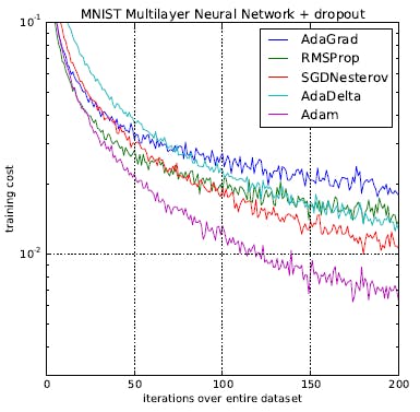
Despite its numerous advantages, it's worth noting that Adam may not always outperform other optimization algorithms in every scenario. For specific problems, other optimizers like SGD with Momentum, RMSprop, or AdaDelta might be more suitable. Proper selection and tuning of optimization algorithms remain important aspects of model training.